Running Exponential Average

Overview

In conventional transport modelling, turbulent fluxes are modelled in terms of processes which are diffusive in the local relaxation sense, with the average flux given by a diffusion coefficient and an effective pinch velocity. The equations are of dominantly parabolic character, which means in practice that an iterate will move monotonically towards the solution in parameter space.

This is not the case for turbulence. Convergence is statistical, which is something different than a diffusive relaxation. If turbulence is stationary, it is meant only that the mean of a distribution of iterates is stationary, not the iterates themselves. The standard deviation can be significant, of order unity compared to the mean, of any distribution of iterates.

This makes for a noisy signal if the output of a turbulence code is used for transport coefficients in a workflow. A sound way to overcome the attendant problems is to use a moving average. Even an average over a moving window can be as noisy as the original signal, however. What works better is a weighted average over recent past values. A method to get this is called a running exponential average, which is essentially the same thing as a convolution integral over an exponential memory decay times the past signal. It turns out to be very easy to obtain this without saving past values.

The original reference for the following is S W Roberts, "Control Chart Tests Based on Geometric Moving Averages," Technometrics1 (1959) 239-250, cited by all the good WWW resources, including the Wikipedia page on Moving Averages and the NIST Statistical Handbook online.

Definition

Consider a process which is a functional of dependent variables Measure at discrete time intervals with values and interval length The moving exponential average on the interval is defined as

in which the small parameter is given in terms of the interval and an inverse time constant

In the first instance is measured there is no so the first value of is simply set to since it can be assumed that the initial state for has persisted for infinite previous time up to the initial time point.

Differential Equation

The equivalent differential equation is found by forming the relevant finite difference,

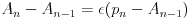
which we can also cast as Taking the limit is the same as taking so both of these expressions become equivalent to whose solution is given below.

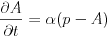
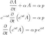
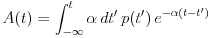
Equivalence to Past-Time Convolution Integral

The solution of the above differential equation is given by the method of undetermined coefficients,

We may integrate this over all past time, to find This is a convolution integral over the kernel and the signal The time constant is just the memory decay time, while if is constant then the integral yields unity times This is the same as the normalisation with the factor in the average formula above, which is needed since the interval is of finite size.

Hence the running exponential average is operationally the same as a memory decay integral over past time. The elegant feature is the need to keep only the current value of as it already contains all that is needed of the past time evolution of

notes

Some properties of the running exponential average and how to choose its main time-memory parameter:

• The factor is needed for normalisation
• if then for all
  • the integral with yields unity
  • the and factors add to unity
  • therefore set the first value of to the first value of

• in choosing the memory decay time
  • one should have
  • best results are for
  • some trial/error required; edge turbulence likes

In these expressions and are the correlation and saturation times of the turbulence, respectively.